Playing and Recording Audio Files

The scipy.io.wavfile library allows us to deal with WAV files. For instance, given the following recording of the note Do,

we can load it into Python as follows:

>>> from scipy.io import wavfile
>>> fs, data = wavfile.read('do.wav')
>>> fs
4000
>>> data.shape
(8000,)
>>> data
array([   0,    0,   -1, ...,  -43, -149, -209], dtype=int16)

The wavfile.read() function returns both the sampling frequency of the .wav file ($4000 Hz$ in this case) and a numpy array representing the data read with length 8000 which implies that the recording lasts $2s$.

The fact that the array only has one dimension means that 'do.wav' was a mono sound signal. In the case that it was recorded as a stereo sound signal it the shape of data would have been (8000, 2).

Finally, in order to play or record audio, we can use the PyAudio package which can be installed by means of conda install pyaudio. The main features outlined in its documentation are the following:

To use PyAudio, first instantiate PyAudio using pyaudio.PyAudio(), which sets up the portaudio system.
To record or play audio, open a stream on the desired device with the desired audio parameters using pyaudio.PyAudio.open(). This sets up a pyaudio.Stream to play or record audio.
Play audio by writing audio data to the stream using pyaudio.Stream.write(), or read audio data from the stream using pyaudio.Stream.read().

Provided with this set of tools we can define the following function that allows us to play a numpy array of dtype=int16:

import numpy as np
from scipy.io import wavfile
import pyaudio

def sound(array, fs=8000):
    p = pyaudio.PyAudio()
    stream = p.open(format=pyaudio.paInt16, channels=len(array.shape), rate=fs, output=True)
    stream.write(array.tobytes())
    stream.stop_stream()
    stream.close()
    p.terminate()

When it comes to recording, the function below comes in handy:

def record(duration=3, fs=8000):
    nsamples = duration*fs
    p = pyaudio.PyAudio()
    stream = p.open(format=pyaudio.paInt16, channels=1, rate=fs, input=True,
                    frames_per_buffer=nsamples)
    buffer = stream.read(nsamples)
    array = np.frombuffer(buffer, dtype='int16')
    stream.stop_stream()
    stream.close()
    p.terminate()
    return array

Hence, we are now able to do something like this:

>>> sound(data, fs=4000) # The do note was recorded using a lower sampling frequency of 4000
>>> my_recording = record() # Say something wise
>>> sound(my_recording)

Reading and Visualizing Images

In order to illustrate the discussion of image processing, we have downloaded some classic images for signal processing from the scikit-image repository and saved them in our Python working directory. Indeed, along scikit-image, the main library that we will use is matplotlib.

Moon	Cameraman	Astronaut

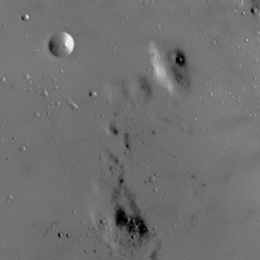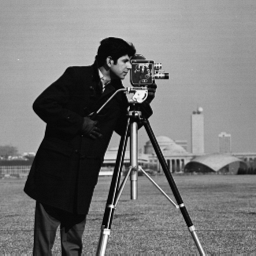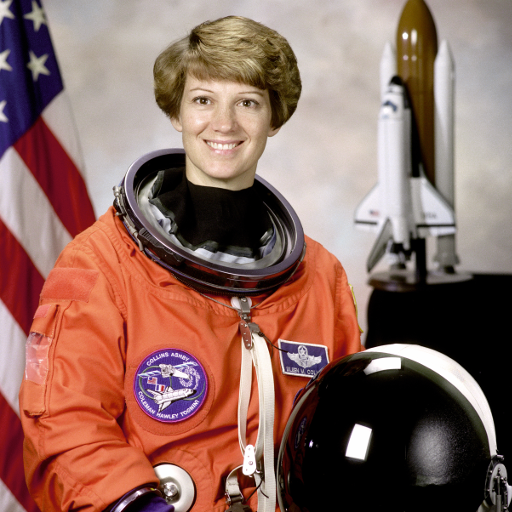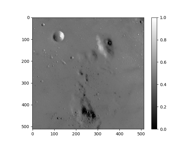
Provided with the function plt.imread() we obtain a numpy array of dimensions (512, 512) that represents our 'moon.png'. image in the range of values $[0, 1]$. Given that it is two-dimensional, it represents a grayscale image.

>>> moon = plt.imread('moon.png')
>>> type(moon)
numpy.ndarray
>>> moon.shape
(512, 512)
>>> moon
array([[0.45490196, 0.45490196, 0.47843137, ..., 0.3647059 , 0.3764706 ,
        0.3764706 ],
       [0.45490196, 0.45490196, 0.47843137, ..., 0.3647059 , 0.3764706 ,
        0.3764706 ],
       [0.45490196, 0.45490196, 0.47843137, ..., 0.3647059 , 0.3764706 ,
        0.3764706 ],
       ...,
       [0.42745098, 0.42745098, 0.4392157 , ..., 0.45882353, 0.45490196,
        0.45490196],
       [0.44705883, 0.44705883, 0.44313726, ..., 0.4627451 , 0.4627451 ,
        0.4627451 ],
       [0.44705883, 0.44705883, 0.44313726, ..., 0.4627451 , 0.4627451 ,
        0.4627451 ]], dtype=float32)

It is relevant to mention that matplotlib can only read the PNG format natively. Provided with a dependency on pillow (which comes installed with Anaconda), we can work with other formats such as JPG or BMP.

In order to visualize the image that we have just loaded we use plt.imshow():

>>> plt.imshow(moon, cmap='gray')
>>> plt.colorbar()
>>> plt.show()

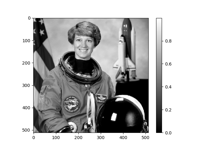
In order to convert an RGB image to grayscale we can use the rgb2gray() function from the skimage.color module which calculates the value of each pixel as the weighted sum of the corresponding red, green and blue pixels as:

Y = 0.2125 R + 0.7154 G + 0.0721 B

Taking the astronaut image as an example:

>>> from skimage.color import rgb2gray
>>> astronaut = plt.imread('astronaut.png')
>>> astronaut.shape
(512, 512, 3)
>>> astronaut_grayscale = rgb2gray(astronaut)
>>> astronaut_grayscale.shape
(512, 512)

Lliçons.jutge.org
Víctor Adell
Universitat Politècnica de Catalunya, 2023