Integration

One-variable integration
Iterated integrals
Numeric integration
Change of variables
External links

One-variable integration

The function from SymPy that we’ll be using for integration is integrate. It’s a very powerful function that can perform many of the common integrals.

Primitives

A primitive of a function $F(x)=\int f(x)dx$ can be computed with:

F = integrate(f, x)

Definite integrals

A definite integral of a function $A = \int_{a}^{b} f(x)dx$ can be computed by adding the upper and lower limits with the variable of integration.

A = integrate(f, (x, a, b))

Improper integrals

Improper integrals $\int_{a}^{\infty}f(x)dx = \lim_{b \to \infty} \int_{a}^{b}f(x)dx$ can be performed just by using th SymPy oo object (infinity) in one or both of the integration limits.

A1 = integrate(f, (x, a, oo))
A2 = integrate(f, (x, -oo, b))
A3 = integrate(f, (x, -oo, oo))

Iterated integrals

As the integrate function returns SymPy functions (or just numbers), they can be called recurively.

For example, a double integration like $A = \int_{a}^{b} dy \int_{c}^{d} f(x)dx$ can be computed calling two times the integrate function.

A = integrate(integrate(f, (y, c, d)), (x, a, b))

📝 Example:

Integrate the function $f(x,y) = x^2 - xy + y^3$ over the domain $D= \left\lbrace (x,y)\in\mathbb{R}^2:1\leq x\leq 2,-2x\leq y\leq x^2 \right\rbrace$
>>> x, y = symbols('x y')
>>> f = x**2 - x*y + y**3
>>> integrate(integrate(f, (y, -2*x, x**2)), (x, 1, 2))
5.3444444444

This method can be used for integrals in any number of dimensions.

💡 Sometimes you will find useful to be able to see the integration domain. Check out the Plotting page to see a full example of it.

Numeric integration

We can also compute integrations using numeric methods with the subpackage integration from SciPy. SciPy is a python package for scientific computation. To use it, we will import it just like any other package:

from scipy import integration

To perform double integrals we will use the function integration.dblquad(). It takes as parameters the function to integrate and the boundaries, and returns the computed value and an estimation of the absolute error.

📝 Example:

Compute the defined integral: $$ \int_{y=0}^{\frac{1}{2}} \int_{x=0}^{1-2y} xydxdy $$
>>> f(x, y):
>>>   return x*y
>>> g(y):
>>>   return 0
>>> h(y):
>>>   return 1 - 2*y
>>> integration.dblquad(f, 0, 0.5, g, h)
(0.010416666666666668, 1.1564823173178715e-16)

⚠️ Warning: The boundaries type must be float or callable objects (basically functions).

💡 All the parameters of the previous example passed as functions can also be passed as lambda functions. Here is how it could be done in a single line:
dblquad(lambda x, y: x*y, 0, 0.5, lambda x: 0, lambda x: 1-2*x)
For more information about lambda functions check out this w3school page

To compute triple integrals we can use the function integration.tplquad(). It works exactly in the same way as the previous function but it takes two extra parameters for the two extra boundaries.

Change of variables

The Matrix class has a method called jacobian to compute the jacobian of a matrix. It takes a list of variables as a parameter.

x1, x2, ... xn = symbols('x1 x2 ... xn')
M = Matrix( ... )
M.jacobian([x1, x2, ... xn])

📝 Example:

Compute the integral of the function $\sqrt{x^2+y^2}$ over the annulus $D = \left\lbrace (x,y)\in\mathbb{R}^2 : 4 \leq x^2 + y^2 \leq 9 \right \rbrace$
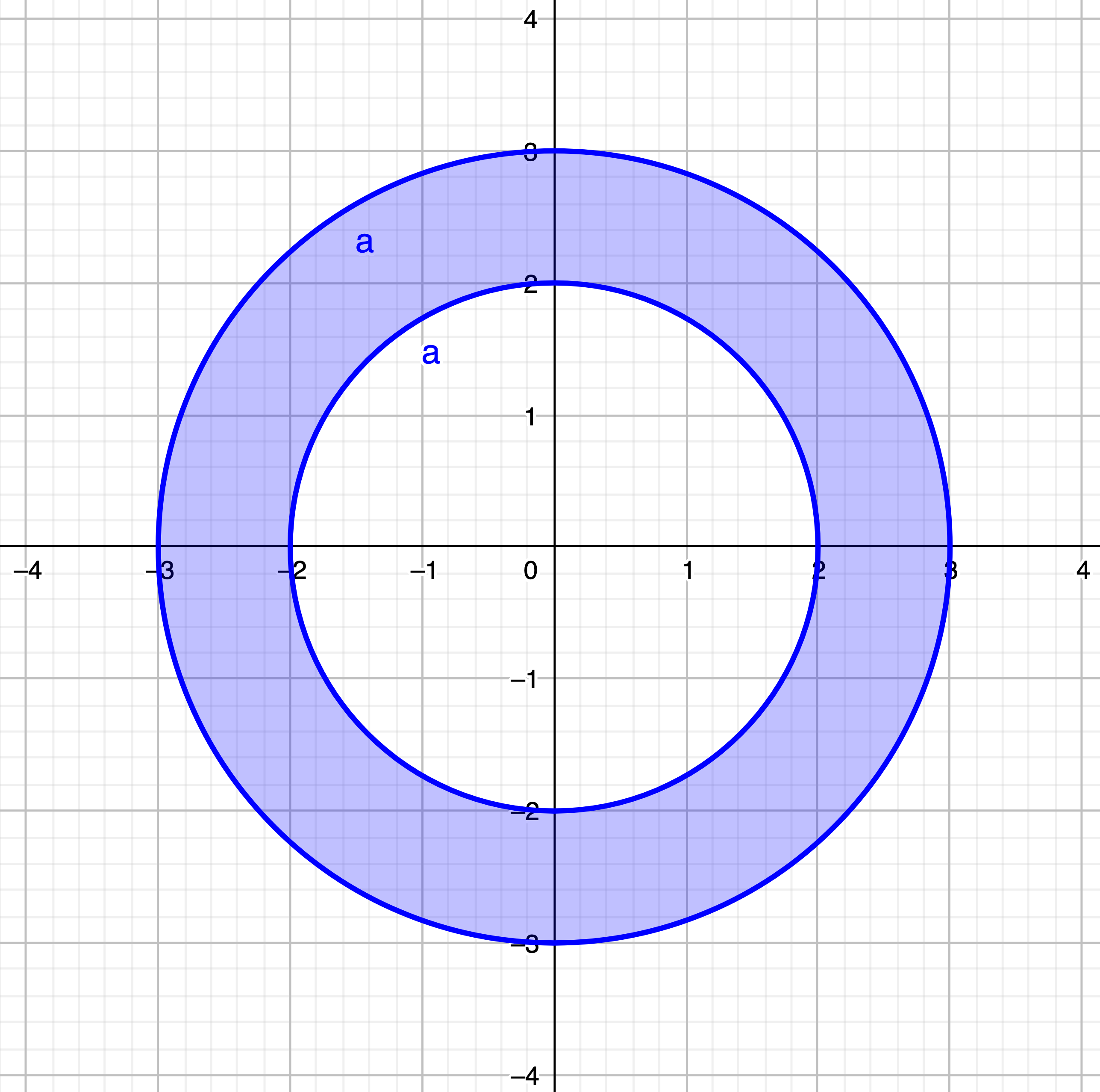
>>> r, alpha = symbols('x y r alpha')
>>> x = r*cos(alpha)
>>> y = r*sin(alpha)
>>> f = sqrt(x**2 + y**2)
>>> J = Matrix([x, y]).jacobian([r, alpha])
>>> integrate(integrate(f*abs(J.det()), (alpha, 0, 2*pi)), (r, 2, 3))
38*pi/3
👁️ Note: (cos, sin, sqrt and pi are functions and objects from the SymPy package)

External links

Lliçons.jutge.org
Raúl Higueras
Universitat Politècnica de Catalunya, 2023